Spectrum

Introduction

Every sound you hear is a cocktail of frequencies — bass, midrange, treble — mixed together into a single pressure wave. A spectrum analyser takes that wave apart, revealing its ingredients in real time. This article explains how Spectrum does it: capturing audio from the iPhone's microphone, decomposing it with a Fast Fourier Transform, and rendering the result at 60 frames per second using the GPU.

The architecture splits neatly into two halves. The audio pipeline runs on the CPU, using Apple's Accelerate framework to perform signal processing with SIMD instructions — processing four or eight numbers simultaneously on every clock cycle. The rendering pipeline runs on the GPU via Metal, turning frequency data into coloured triangles that the hardware rasterises in parallel across thousands of shader cores.

Between these two halves sits a crucial design decision: decoupled rates. Audio arrives at ~21 frames per second (every 2048 samples at 44.1kHz). The display runs at 60 frames per second. Rather than coupling them — which would mean either wasting GPU frames or stuttering the animation — the renderer maintains its own smoothed state and interpolates toward the latest audio data on every frame. This is what gives the display its fluid, professional feel.

What follows is a complete walkthrough of both pipelines, from microphone to pixel, with the mathematics behind each stage and how those operations map to the hardware.

Part 1: The Audio Pipeline

The journey from microphone to frequency data passes through eight stages, each performing a well-defined mathematical operation. What makes this fast isn't clever algorithms alone — it's that Apple's Accelerate framework maps each operation onto SIMD (Single Instruction, Multiple Data) instructions. ARM NEON, the SIMD engine on Apple Silicon, processes 4 floats simultaneously in a single clock cycle. The entire pipeline completes in about 10 microseconds — 0.02% of the available time budget.

1. Windowing — Reducing Spectral Leakage

The microphone delivers a continuous audio stream, but the FFT operates on a finite chunk (2048 samples). Abruptly cutting the signal at chunk boundaries creates artificial high-frequency artefacts called spectral leakage. A Hanning window tapers the signal to zero at both edges, eliminating this.

2. Packing — Real Data to Split Complex Format

The vDSP FFT requires input in split complex format: separate arrays for real and imaginary parts. Since our audio is purely real (no imaginary component), we pack it by treating consecutive pairs of real samples as (real, imaginary) pairs.

3. FFT — Time Domain to Frequency Domain

The Discrete Fourier Transform decomposes a time-domain signal into its constituent frequencies. For N samples, the DFT is:

Naively, this is O(N²) — each of the N output bins sums over all N input samples. The Fast Fourier Transform (Cooley-Tukey algorithm) exploits symmetries in the twiddle factors e^(−j2πkn/N) to reduce this to O(N log N). For N=2048, that's ~22,000 operations instead of ~4.2 million.

4. Squared Magnitudes — Complex to Power

The FFT output is 1024 complex values. We need the power (squared magnitude) at each frequency — this tells us how much energy is present at that frequency.

5. Power to Decibels — Logarithmic Scaling

Human hearing perceives loudness logarithmically — a 10× increase in power sounds roughly "twice as loud". Converting to decibels maps this perception to a linear scale.

Values are floored to 10⁻²⁰ before the log to avoid −∞ from silent bins.

6. Logarithmic Band Mapping — Perceptual Frequency Grouping

The 1024 FFT bins are linearly spaced in frequency (each bin = sampleRate/N ≈ 21.5 Hz). But human pitch perception is logarithmic — the jump from 100 Hz to 200 Hz (one octave) sounds the same as 1000 Hz to 2000 Hz (also one octave). We map bins to 128 logarithmically-spaced bands.

This is implemented as a scalar loop since each band maps to a different number of bins — not a uniform SIMD operation. At only 128 iterations with simple averaging, it completes in microseconds.

7. Auto-Leveling & Normalisation

Rather than mapping a fixed -80 to 0 dB range (which leaves quiet signals invisible), the display window adapts to the current signal level. The ceiling tracks the peak dB value with instant rise and slow decay.

8. 60fps Smoothing & Peak Tracking (in Renderer)

The audio engine publishes raw normalised data at ~21fps. The Metal renderer applies its own smoothing at 60fps for silky-smooth animation, completely decoupled from the audio update rate.

Asymmetric exponential smoothing — fast attack, slow decay:

Peak tracking at 60fps — instant rise, gentle fall:

Performance Summary

The entire audio pipeline uses roughly 0.02% of the available CPU budget per audio callback — demonstrating why vDSP's SIMD approach is more than adequate and GPU compute would add complexity for no benefit at this scale.

Part 3: System Architecture

The view hierarchy, data flow, rendering pipeline, and testing infrastructure that connect the audio and rendering halves into a working app.

Part 2: The Rendering Pipeline

At this point we have 128 normalised frequency values arriving ~21 times per second. The rendering pipeline's job is to turn these numbers into a beautiful, fluid visualisation at 60 frames per second — smoothing over the gaps between audio updates and giving the user four distinct ways to see their sound.

Why Metal, Not SwiftUI

SwiftUI is excellent for UI controls (our mode picker and label overlays use it), but for rendering thousands of animated shapes at 60fps it becomes a bottleneck. Each SwiftUI view carries overhead — identity tracking, diffing, layout computation. Drawing 128 animated bars means 128 view updates per frame through SwiftUI's reconciliation engine.

Metal bypasses all of this. We write vertex data directly into GPU memory and issue a single draw call. The GPU's massively parallel architecture rasterises all triangles simultaneously. For our spectrogram mode with ~98,000 triangles, this is the difference between fluid animation and a slideshow.

The Single-Pipeline Architecture

All four visualisation modes share one Metal render pipeline — a single vertex shader and a single fragment shader. Rather than writing mode-specific GPU code, we do the mode-specific work on the CPU: building an array of coloured triangles that the GPU simply renders. This is the key architectural choice.

This works because our bottleneck is fill rate (pixels), not vertex throughput. Modern mobile GPUs can handle millions of vertices per frame — our maximum of ~100K is trivial. The simplicity of having one shader pair means less GPU state switching, fewer pipeline objects, and dramatically simpler code.

Vertex Layout and the Alignment Lesson

Each vertex is a Swift struct with a 2D position and an RGBA colour:

The Metal shader must use matching types. Using packed_float4 (no alignment padding, 24-byte stride) caused a critical bug — every vertex after the first was read from the wrong offset, producing garbled geometry. The fix was to use non-packed float2/float4 in Metal, giving the same 32-byte stride with identical padding.

How Each Mode Builds Geometry

Bars Mode

The classic equaliser. Each of the 128 frequency bands becomes a vertical rectangle (quad), rendered as two triangles. Colour is determined by frequency position through a five-stop gradient ramp.

Curve Mode

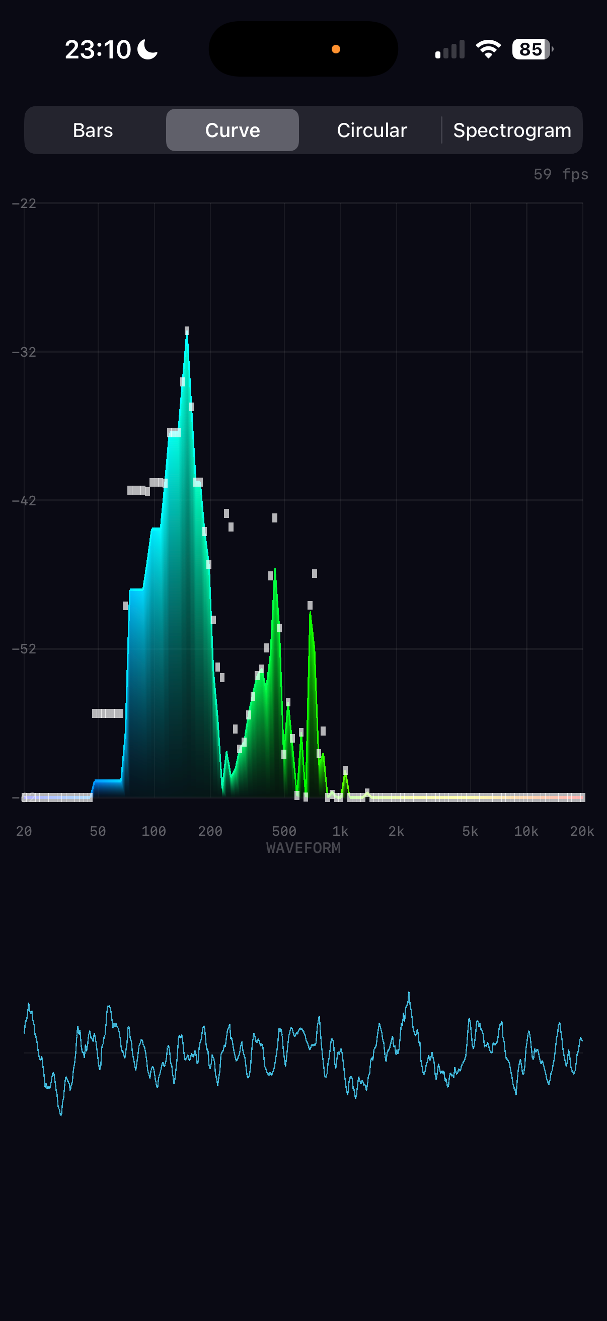
A smooth filled area under the frequency curve, with a bright outline traced along the top edge.

Circular Mode

Frequency bands radiate outward from a central point, creating a pulsing ring. Each band is a tapered bar at a specific angle around the circle.

Spectrogram Mode

A scrolling heatmap where the x-axis is frequency, the y-axis is time, and colour represents intensity. This is the most vertex-heavy mode.

Waveform (All Modes)

The time-domain audio signal rendered as a cyan trace below the spectrum area. Drawn as a series of thin quads along the waveform curve, similar to the curve outline technique.

60fps Asymmetric Smoothing

A critical insight: the audio engine delivers new spectrum data at ~21fps (every 2048 samples at 44.1kHz), but the display runs at 60fps. If we used the audio data directly, bars would jump 21 times per second with dead frames in between — visible as micro-stuttering.

The renderer maintains its own displaySpectrum array and interpolates toward the target on every frame:

Why asymmetric? Equal attack and decay feels "mushy" — sounds seem to linger too long. Fast attack captures transients like drum hits instantly, while slow decay creates a smooth, natural fade that reads as "energy dissipating" rather than "signal dropping". The ~3:1 ratio between attack and decay is common in professional audio metering.

Peak tracking also runs at 60fps — peaks snap up instantly but fall at 0.006/frame, taking ~3.5 seconds to fully decay. This creates the characteristic "falling dot" effect seen in professional analysers.

The Draw Call

After building all vertices (spectrum + waveform), the renderer uploads them to the GPU and issues one draw call:

Rendering Performance

The GPU handles the heavy lifting — rasterising triangles, interpolating colours, and blending with alpha transparency. The CPU's job is just to decide what to draw and where. This CPU-for-logic, GPU-for-pixels split is the same principle behind every real-time graphics application, from games to medical imaging.

Part 4: Pitch Detection — Time-Domain Autocorrelation

A spectrum analyser shows what frequencies are present in a signal. A tuner goes further: it identifies the single fundamental pitch the listener perceives — the note a musician is playing — and tells them how far sharp or flat they are. This turns out to be a surprisingly subtle problem, and the solution that works robustly for real voices and instruments is a direct, time-domain approach: computing autocorrelation from the raw audio samples themselves.

The Problem: Why the Loudest Bin Is Not the Pitch

The naive approach — "find the FFT bin with the highest magnitude and call that the pitch" — fails for almost every real instrument. The reason is harmonics. When a guitar plays A4 (440 Hz), the string vibrates not just at 440 Hz but simultaneously at 880, 1320, 1760 Hz and beyond. These are integer multiples of the fundamental, and for many instruments and the human voice, the second or third harmonic is louder than the fundamental itself.

There is a second problem: frequency resolution. With a 2048-sample FFT at 44100 Hz, each bin spans 44100/2048 = 21.5 Hz. The semitone above A4 is Bb4 at 466.2 Hz — a gap of just 26.2 Hz, barely more than one bin width. At lower pitches the problem is worse: the semitone from E2 (82.4 Hz) to F2 (87.3 Hz) is only 4.9 Hz, meaning several notes share the same FFT bin. Simply reading bin indices cannot achieve the sub-hertz accuracy a musician needs.

We need a method that finds the period of the fundamental — the common spacing between all harmonics — regardless of which harmonic is loudest, and with much finer resolution than the FFT grid allows.

Autocorrelation: Finding Periodicity

The key insight is that a periodic signal, when compared with a time-shifted copy of itself, will show maximum similarity at a shift (or lag) equal to one full period. This self-similarity measure is called autocorrelation.

Imagine photocopying a waveform onto a transparency and sliding it over the original. At zero offset, every peak aligns — perfect correlation. As you slide, alignment degrades. But when you shift by exactly one period, peaks align again. The lag at this alignment is the fundamental period, and the frequency is simply 1/period.

Why Not Wiener-Khinchin? A Development Journey

The initial implementation used the Wiener-Khinchin theorem, which computes autocorrelation as the inverse FFT of the power spectrum: R[L] = IFFT(|X[k]|^2). This was mathematically elegant and computationally efficient — the power spectrum was already available from the visualiser pipeline, so pitch detection cost just one additional IFFT (~5 microseconds). It worked beautifully for pure test tones.

However, the Wiener-Khinchin approach failed badly for real voice and instruments. The root cause: squaring the power spectrum exaggerates harmonics. When the power spectrum is squared (|X[k]|^2 becoming |X[k]|^4 in effect), already-strong harmonics become disproportionately dominant. For a human voice where the second harmonic is naturally louder than the fundamental, the squaring makes the sub-harmonic peak at lag=2T (one octave low) competitive with or stronger than the true peak at lag=T. The result was wild octave errors and instability — the detected pitch would jump erratically between the correct note and one octave below.

The solution was to abandon the frequency-domain shortcut entirely and compute autocorrelation directly from the time-domain audio samples, using Pearson-normalised correlation that treats each lag independently.

Time-Domain Autocorrelation with Pearson Normalisation

For each candidate lag L, we compute the Pearson correlation coefficient between the original signal segment x[0..n-L] and the shifted segment x[L..n]. Unlike the raw dot product (which depends on signal energy and decreases at longer lags), the Pearson coefficient is normalised to the range [-1, 1], making it directly comparable across all lags:

Incremental energy update: The naive approach recomputes both segment energies from scratch for every lag — O(N) work per lag, O(N^2) total. Instead, the segment energies are updated incrementally: as the lag advances from L to L+1, one sample leaves the left segment and one enters the right segment. Each energy update is O(1): subtract the departing sample's squared value, add the arriving sample's squared value. This reduces the inner loop to a single vDSP_dotpr call plus two additions per lag.

First-peak search: The search scans from high frequency to low (starting at 1000 Hz, i.e. short lags) and returns the first peak above the 0.75 confidence threshold — not the global maximum. This is critical for avoiding sub-harmonic errors: the autocorrelation always has a peak at 2T (the second period) that can be stronger than the peak at T for complex timbres. By searching from short lags upward and stopping at the first confident peak, the algorithm naturally finds the fundamental period rather than a sub-harmonic.

Parabolic Interpolation: Sub-Sample Precision

The autocorrelation gives us one value per integer lag — one per sample. At 44100 Hz, the lag for A4 (440 Hz) is 44100/440 = 100.23 samples. The nearest integer lags are 100 and 101, corresponding to frequencies 441.0 Hz and 436.6 Hz respectively — a difference of 4.4 Hz, which is 17 cents (nearly a fifth of a semitone). A musician needs accuracy of 1-2 cents.

The solution is parabolic interpolation: fit a parabola through the peak sample and its two neighbours, then find the true peak of the parabola. This yields sub-sample accuracy from integer-spaced data.

This is the same technique used in professional tuners. The parabolic fit costs three multiplies and two divides — negligible compared to the autocorrelation loop — but converts bin-level resolution into the sub-hertz accuracy musicians require.

Musical Note Conversion

Once we have a precise frequency, converting to a musical note name involves logarithmic maths and a lookup table. Western music divides the octave into 12 equal semitones, where each semitone is a frequency ratio of 2^(1/12) = 1.05946. The reference point is A4 = 440 Hz.

Confidence and Smoothing

Not every audio frame contains a clear pitch. Background noise, breath sounds, percussive hits, and polyphonic passages all produce autocorrelation functions without a dominant peak. Displaying a wildly flickering note name in these situations is worse than displaying nothing.

Confidence metric: The Pearson correlation coefficient at the detected peak directly measures how periodic the signal is. A pure sine wave gives close to 1.0; white noise stays near 0. With Pearson normalisation, the threshold for a "confident" pitch detection is 0.75. This cleanly separates pitched signals from noise: human voice typically produces peaks of 0.93 or higher, while background noise rarely exceeds 0.68. The high threshold eliminates the false detections that plagued the earlier Wiener-Khinchin approach.

Median filtering over averaging: Pitch estimates are subject to occasional octave errors — the autocorrelation can lock onto a sub-harmonic, producing a reading one octave low. A simple moving average would blend these errors into the result, producing a pitch that is neither correct nor one octave off — just wrong. A median filter (over 3 frames, ~144ms) rejects these outliers cleanly: if 2 out of 3 frames read 440 Hz and one reads 220 Hz, the median is 440 Hz. The octave jump is discarded entirely. The shorter 3-frame window (compared to the 5-frame window used in the earlier implementation) provides faster response while the Pearson normalisation's inherent stability means fewer outliers need filtering.

Colour coding for tuning accuracy:

Part 5: Beat Detection — Spectral Flux and Tempo Estimation

Where pitch detection asks "what note is playing?", beat detection asks "when do rhythmic events happen, and how regularly?" A kick drum, a snare hit, a chord strum — these are onsets: sudden increases in energy that punctuate the flow of music. Detect enough of them, measure the gaps between them, and you have the tempo.

Unlike pitch, which is a frequency-domain question (which frequency dominates?), beat detection is fundamentally about change over time in the spectrum. A steady tone at 100 Hz has no beats. A drum hit at 100 Hz is a sudden appearance of energy at 100 Hz. The distinction lies not in a single FFT frame, but in how consecutive frames differ.

Spectral Flux: Measuring Spectral Change

Spectral flux quantifies how much the spectrum has changed between two consecutive FFT frames. Specifically, it sums the positive magnitude increases across the low-frequency bins where percussive energy concentrates (20-200 Hz). We ignore decreases — a note dying away is not an onset.

The focus on the 20-200 Hz range is deliberate. Kick drums — the rhythmic backbone of most music — concentrate their energy in the 40-100 Hz range. Snare drums have significant energy here too (the body resonance, not just the snap). By ignoring higher frequencies, we avoid false onsets from melodic movement, vocal articulation, and cymbal splashes that do not define the beat.

Onset Detection: Adaptive Thresholding

A raw flux value is meaningless without context. A flux of 50 could be a massive onset in a quiet passage or background noise in a loud one. The threshold must adapt to the recent history of flux values.

The minimum gap of 100 ms corresponds to 600 BPM — far faster than any real music. Its purpose is to prevent a single drum hit, which may cause elevated flux for 2-3 consecutive frames, from being counted as multiple onsets.

Tempo Estimation: Autocorrelation of the Onset Strength Signal

An earlier approach tracked inter-onset intervals (IOIs) from spectral flux peaks: collect onset timestamps, compute the gaps, take the median, convert to BPM. This worked well for straight 4/4 beats but failed completely on syncopated music like drum & bass, where kick drums hit on off-beat subdivisions. The IOI histogram scattered across many wrong tempos (50, 67, 84, 100 BPM) when the true tempo was 123 BPM.

The solution, based on Scheirer (1998) and Ellis (2007), is to autocorrelate the continuous spectral flux signal itself rather than individual onset timestamps. The key insight: even when individual kicks are syncopated, the overall rhythmic pattern repeats at the beat period. Autocorrelation finds this periodicity directly.

Why log compression matters: Raw spectral flux has enormous dynamic range — a loud kick produces flux 100x larger than a quiet hi-hat. Without compression, the autocorrelation is dominated by a few loud events. Log compression (log(1 + 10x)) brings quiet hi-hat onsets to comparable magnitude with loud kicks, making the rhythmic pattern visible across all dynamic levels.

Why detrending matters: Slow energy variations (a crescendo, a quiet intro with harmonic content) create a DC component in the onset signal that produces positive autocorrelation at all lags — resulting in false BPM readings during non-rhythmic passages. Subtracting the 2-second local mean removes these slow variations while preserving the fast rhythmic peaks.

Confidence metric: The ratio of the peak autocorrelation value to the zero-lag (self-correlation) value, after normalisation. The display threshold is 15%. On real music, confidence typically ranges from 37-60% during steady beats — "Missing" at 37-47%, BBC News24 Countdown at 58-61%.

Temporal smoothing: A smoothing buffer of 3 consecutive estimates requires 2 out of 3 to agree within ±5 BPM before the displayed value changes. This prevents brief transient blips from reaching the UI while allowing faster lock-on (~1.5 seconds).

Silence suppression: When the raw flux variance (before detrending) falls below 0.5, no BPM is displayed. This prevents false readings during steady tones and silence where any autocorrelation peak is noise, not rhythm.

Harmonic check with range constraint: After finding the peak lag, the algorithm checks if the half-lag (double tempo) has an autocorrelation peak > 40% as strong. If so AND the resulting BPM would be ≤ 160, the half-lag is preferred. The range constraint prevents incorrect doubling — e.g. a 124 BPM peak at lag 19 must not be doubled to 248 BPM (lag 9) just because lag 9 has some correlation. Results above 160 BPM are auto-halved for display (e.g. D&B at 174 shows as 87).

Tempo-change detection: If 3 consecutive autocorrelation estimates diverge by more than 10 BPM from the currently locked tempo, the entire flux history, smoothing buffer, and onset state are flushed. The detector restarts fresh, typically converging on the correct new tempo within 5-8 seconds. Without this, a wrong initial lock or a track change would persist for 8+ seconds because stale data in the circular buffer keeps reinforcing the old answer. This mirrors the pitch-jump detection in the tuner, which flushes its smoothing buffer when the detected note changes by more than a semitone.

Tested accuracy across 16 commercial tracks: 14 out of 16 tracks detected within ±2 BPM (87.5% accuracy). The algorithm handles a wide range of genres and tempos: Get Lucky (116→116), Sledgehammer (96→97), Rock DJ (103→104), Down Under (107→108), Running Up That Hill (108→109), Relax (115→115), Don't You Want Me (118→119), BBC News24 (120→120), Sussudio (121→121), One More Time (122→123), Missing (123→124), Rhythm of the Night (128→127), Canned Heat (128→128), Video Killed the Radio Star (132→131).

Beat Flash Visualisation

Detected beats are communicated visually through a brief brightness flash on the spectrum visualisation — a subtle but satisfying pulse that confirms the algorithm is tracking the rhythm. The flash is designed to feel instantaneous and natural, like a light reacting to a drum hit.

Performance Budget

Beat detection runs alongside the existing FFT visualisation pipeline and the optional pitch detection. The key question is whether the combined DSP load fits comfortably within the audio callback budget.

Part 6: 3D Surface Rendering

The first four visualisation modes (bars, curve, circular, spectrogram) are all 2D — they plot frequency data in screen space using flat coloured triangles. The surface mode adds a third dimension: time flows into the screen as a scrolling mesh, with amplitude forming a terrain-like surface lit by a directional light. This requires a fundamentally different rendering pipeline.

Dual Pipeline Architecture

A natural question: why not extend the existing 2D pipeline to handle 3D as well? The answer comes down to vertex bandwidth. The 2D modes process up to 100,000 vertices per frame, each at 32 bytes (position SIMD2<Float> + colour SIMD4<Float>). Adding normals for lighting would inflate every vertex to 48 bytes — an extra 1.6MB of GPU bandwidth per frame — even though the 2D modes never use normals. Conversely, the 3D surface mode processes ~45,000 vertices (or ~91,000 with ridgelines in surface+ mode) but needs normals for lighting and a uniform buffer for the model-view-projection matrix, neither of which the 2D pipeline requires.

The clean solution is two separate MTLRenderPipelineState objects, each with its own vertex descriptor and shader pair. They share the same MTKView and command queue — only the pipeline state and vertex buffer format differ.

Both pipelines are created once at init time. Each frame, the renderer checks the current mode and selects the appropriate pipeline state, vertex buffer, and draw call. The 2D pipeline uses no depth buffer (painter's algorithm with draw order). The 3D pipeline enables depth testing and writes to a depth texture attached to the render pass.

3D Vertex Structure

The surface vertex layout is driven by Metal's alignment requirements. Metal's float3 and Swift's SIMD3<Float> both occupy 16 bytes (12 bytes of data, 4 bytes of padding to align to 16-byte boundaries). This alignment is mandatory — mismatched strides between Swift and Metal cause garbled geometry.

MVP Matrix Construction

The 3D surface uses an orbit camera — the camera sits on the surface of a sphere centred on the origin, parameterised by azimuth (horizontal angle), elevation (vertical angle), and distance. The user's view is fixed (no interactive rotation), but the camera position is computed dynamically to adapt to different aspect ratios.

Aspect-Ratio-Adaptive Camera

The Metal view's height changes depending on the UI state: full height in mic mode, reduced height when the transport bar is visible, and further reduced when the music browser is open. This means the aspect ratio varies significantly. A fixed camera that looks good in one state clips the mesh or leaves dead space in another.

The solution is two camera presets — one tuned for tall/narrow views (compact mode, closer camera, steeper elevation) and one for wide/short views (full mode, farther camera, shallower elevation). The actual camera parameters are smoothly interpolated between these presets based on the current aspect ratio.

Directional Lighting

The surface uses a simple Lambertian diffuse lighting model — the brightness of each fragment depends on the angle between the surface normal and the light direction. This is the simplest physically-motivated lighting model: a surface facing the light is fully lit, a surface perpendicular to the light receives no direct illumination, and an ambient term prevents unlit faces from going completely black.

Surface Mesh Generation

The surface mesh is a scrolling grid: frequency maps across the X axis and time flows along the Z axis. A circular buffer of 60 rows stores the spectrum history (~3 seconds at 20fps update rate). Each audio frame, the newest spectrum data is written into the current row and the write index advances. The mesh generator reads all 60 rows, wrapping around the buffer, to produce a continuous surface.

The adaptive Y scale ensures the surface amplitude is visually proportional to the available view height. In compact mode (browser open, aspect ratio below 0.55), the scale is clamped to 0.6 to prevent the peaks from overflowing the viewport. In full view (mic mode, aspect ratio above 0.75), the scale extends to 1.2 for more dramatic peaks.

Ridgeline Outlines (Surface+ Mode)

Inspired by curve mode's bright top-edge outline, the surface+ mode adds thin ridgeline outlines traced along the top edge of each time row. These outlines give the mesh a wireframe-like definition that makes individual spectrum snapshots visually distinct as they scroll into the distance.

Performance

The 3D surface mode sits comfortably within the existing performance budget. The vertex count is well below the 2D modes, and the additional cost of depth testing and normal computation is negligible on modern Apple GPU architectures.