Spectrum
Build Tutorial — A conversation-driven development narrative
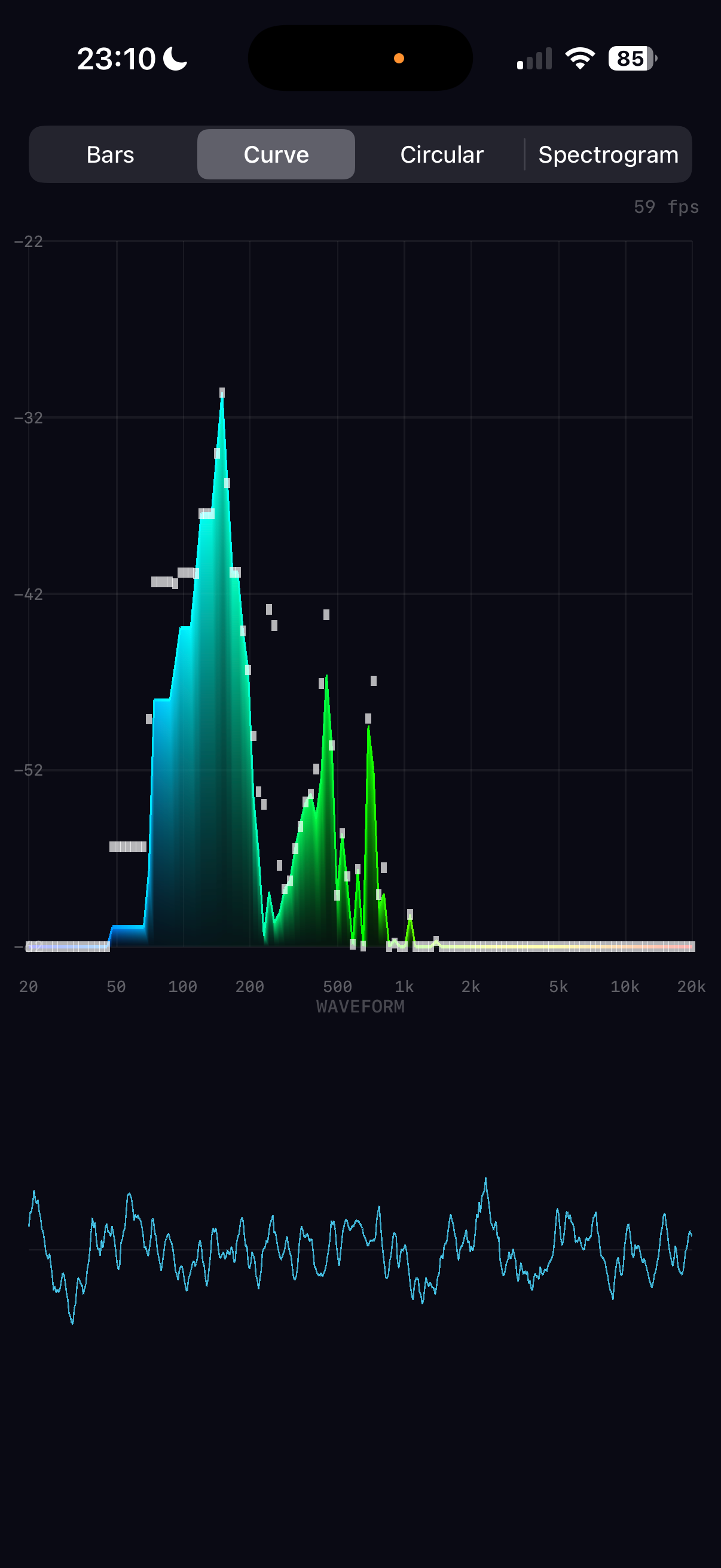
The finished app running on iPhone 16 Pro — built entirely through conversation
1
The Initial Vision
I'd love to build a real-time audio spectrum analyser that shows a beautiful real-time display on my phone of the live frequency breakdown of incoming audio. Could we utilise the GPU for graphics, and would it be worth using it for the audio analysis too — presumably a fast Fourier transform?
The key architectural decision was made upfront: use the GPU (Metal) for rendering but the CPU (Accelerate/vDSP) for FFT analysis. Apple's vDSP is heavily SIMD-optimised and processes a 2048-sample FFT in microseconds. Running FFT on the GPU via Metal compute shaders would add complexity with data-transfer overhead that negates any speed benefit at these buffer sizes. The GPU's strength is rendering thousands of coloured triangles per frame — exactly what we need for the visualisation.
The decision to use vDSP over Metal compute is buffer-size dependent. For audio (1K–4K samples), CPU wins. For large-scale signal processing (millions of samples), GPU compute would be worth the transfer overhead.
2
Clarifying the Design
Multiple visualisation modes please. Gradient colours (cool to hot). Logarithmic frequency scale. Peak indicators, dB scale, frequency labels, waveform view beneath. Let's call it Spectrum.
With clear requirements established, the full architecture was planned: four modes (Bars, Curve, Circular, Spectrogram), all rendered through a single Metal pipeline using coloured triangles. The audio engine would capture via AVAudioEngine, process with vDSP, and publish normalised data that the renderer reads each frame.
Complete project scaffolded in one pass: 7 Swift source files, 1 Metal shader file, Xcode project, and all documentation. The build succeeded on the first attempt — a testament to careful upfront planning of the pbxproj structure and Metal pipeline configuration.
3
The Audio Pipeline
The FFT pipeline was built using Accelerate's C-level vDSP functions rather than the newer Swift overlay, giving precise control over the processing chain:
Hanning window → reduces spectral leakage at buffer boundaries
vDSP_ctoz → packs real audio data into split-complex format
vDSP_fft_zrip → performs the real-to-complex FFT in-place
vDSP_zvmags → computes squared magnitudes (power spectrum)
vDSP_vdbcon → converts power to decibels
The logarithmic band mapping is critical for musical perception. Linear mapping would dedicate half the display to frequencies above 10kHz (one octave), while log mapping gives equal visual weight to each octave: 20–40Hz, 40–80Hz, ..., 10k–20kHz. This matches how we actually hear pitch.
4
Metal Rendering Architecture
Rather than using separate Metal pipelines for each visualisation mode, all four modes share a single vertex/fragment shader pair. The CPU builds coloured vertex data (position + RGBA) each frame, uploads it to a pre-allocated 200K-vertex Metal buffer, and issues a single draw call. This keeps the shader code trivial while giving full flexibility on the CPU side.
The spectrogram mode was initially considered with a Metal texture approach, but the vertex-based approach (128×128 coloured quads = ~98K vertices) proved simpler and well within performance budgets.
The gradient colour scheme maps frequency position (0–1) through a five-stop ramp: blue → cyan → green → yellow → red. This provides good perceptual contrast across the spectrum. The spectrogram uses a separate heatmap that starts from black for silence, making quiet regions visually distinct.
5
The Metal Alignment Bug
The graphics seem broken. Are you able to test in the simulator? Also once you choose Spectrogram the app freezes.
The root cause was a struct alignment mismatch between Metal and Swift. The Metal shader used packed_float2 + packed_float4 (24 bytes per vertex, no padding), but Swift's SIMD4<Float> requires 16-byte alignment, making SpectrumVertex 32 bytes (with 8 bytes of padding between position and colour). Every vertex after the first was read from the wrong offset, causing garbled positions and colours.
In Spectrogram mode, the ~98K triangles with garbled positions created degenerate geometry covering the entire screen many times over, overwhelming the GPU with fragment shader work — causing the freeze.
Changed the Metal shader to use non-packed float2/float4 types, matching Swift's 32-byte stride. Also added reserveCapacity for the vertex array and throttled spectrogram history updates to ~20fps. All four modes now render correctly with no freezing.
This is a common Metal/Swift pitfall. Metal's packed_float4 has 4-byte alignment (24-byte struct), while Swift's SIMD4<Float> has 16-byte alignment (32-byte struct). Always verify that Metal struct layouts match Swift struct layouts — MemoryLayout<T>.stride is the key value to check.
6
Simulator Testing with Launch Arguments
You don't need to guess where the UI buttons are — you can add command line args to set the mode of operation when testing! This is how we eventually got the ShiftingSands simulation working, if you remember?
Rather than trying to tap simulator UI from the command line (which is unreliable), the app was given launch argument support. ProcessInfo.processInfo.arguments is parsed in ContentView to accept -mode bars|curve|circular|spectrogram. This enables fully automated visual testing: install, launch with a specific mode, screenshot, verify — all from the command line.
All four modes were tested automatically in the simulator, confirming correct rendering after the alignment fix. The pattern was documented in the top-level CLAUDE.md as a standard approach for all future projects with multiple visual states.
The testing workflow: xcrun simctl terminate → xcrun simctl launch ... -- -mode X → sleep 2 → xcrun simctl io screenshot. Grant permissions upfront with xcrun simctl privacy ... grant microphone to avoid dialogs.
7
Comprehensive Test Suite
Don't forget to write comprehensive tests!
Pure decision logic was extracted from AudioEngine and MetalRenderer into internal static methods that can be tested without audio hardware or a Metal GPU. This included logarithmic band mapping, exponential smoothing, peak tracking, gradient colour calculation, and heatmap colour mapping. The test target uses Xcode 16's PBXFileSystemSynchronizedRootGroup for automatic test file discovery.
46 tests across three suites (AudioEngineTests, MetalRendererTests, SpectrumDataTests) covering boundary values, clamping, interpolation, colour stops, layout constraints, coordinate conversion, and custom dB range parameters. All passing.
8
Mic Sensitivity and Auto-Leveling
I think we need more sensitive auto-scaling — it's still hard to get much of a display. Maybe the processing mode is only getting a quiet signal from the mic?
Three issues were identified working together to suppress the display:
1. Audio session mode: .measurement mode disables the iPhone's automatic gain control, resulting in very quiet raw mic input. Switching to .default mode enables AGC for maximum sensitivity.
2. FFT normalisation: The power spectrum was normalised by 1/N², but for a one-sided spectrum (discarding the symmetric negative frequencies) the correct factor is 4/N² — a +6dB boost.
3. Auto-level too conservative: The minimum ceiling of -30dB was too high, and the 60dB display range too wide. Changed to ceiling [-60, 0] with a 40dB window for much more visual sensitivity.
The display now fills with activity even in a quiet room. dB labels update dynamically to show the current auto-leveled range, confirming the adaptation is working.
9
60fps Smoothing and FPS Counter
Could we have an FPS display in the corner of the screen? I'm hoping the decay of the display can be ultra-smooth pro graphics quality.
The fundamental issue was that smoothing happened at the audio callback rate (~21fps), not the display rate (60fps). Bars would jump 21 times per second with dead frames in between — visible as micro-stuttering.
The fix was to decouple the animation from the audio pipeline entirely. AudioEngine now publishes raw normalised spectrum data. MetalRenderer maintains its own displaySpectrum array and interpolates toward the target values every frame at 60fps using asymmetric lerp — fast attack (0.35) for responsive rises, slow decay (0.12) for smooth, professional-quality falls. Peak tracking also moved to 60fps with a gentle 0.006/frame decay (~3.5 seconds for a full fall).
An FPS counter was added by tracking frame times in the renderer and displaying via a SwiftUI overlay that polls the shared coordinator every 0.5 seconds.
The display runs at a locked 60fps with silky-smooth bar rises and falls. The decoupled architecture means even if the audio callback rate varies, the animation quality is consistent.
Asymmetric smoothing is key to professional audio visualisers. Equal attack and decay feels "mushy" — sounds seem to linger too long. Fast attack (0.35) captures transients like drum hits instantly, while slow decay (0.12) creates a smooth, natural fade that reads as "energy dissipating" rather than "signal dropping". The 3:1 ratio between attack and decay is a common starting point in pro audio metering.
10
Architecture as a Technical Article
Could you make architecture.html something more like an article I would read in a technical magazine? Nice intro, explanation of the narrative... and could you add inline diagrams and images? The DSP sections aren't very clear to read — could you format them better?
The architecture document was transformed from a flat reference into a three-part technical article. A magazine-style introduction sets the scene — what a spectrum analyser does, why the architecture splits into CPU audio and GPU rendering, and the key insight about decoupled rates.
The math blocks were completely restyled with colour-coded syntax: cyan for variables, purple for functions, green for numbers, orange for operators, blue headings for visual hierarchy, and proper HTML tables replacing monospaced columns. Inline SVG diagrams were added throughout — a Hanning window visualisation, a time-to-frequency domain transform, a linear-vs-logarithmic band comparison, an auto-leveling before/after, a CPU/GPU pipeline split, gradient colour ramps, a memory alignment bug diagram, and a full-colour spectrogram heatmap simulation.
The architecture document now reads as a self-contained article explaining how to build a real-time spectrum analyser, from microphone to pixel. Each mathematical concept is introduced with context, visualised with a diagram, expressed with formatted equations, and grounded with the specific vDSP function and NEON instruction count that implements it.
11
Music Playback Mode
The list of songs contains many that won't play. Could we filter out DRM-protected tracks and add a music playback mode with spectrum analysis?
Music playback required a second audio path through AVAudioEngine: AVAudioPlayerNode → AVAudioMixerNode (with FFT tap) → mainMixerNode. The mixer tap feeds the same FFT pipeline as the mic, so all four visualisation modes work identically with music.
The music library is loaded via MPMediaQuery.songs() with DRM filtering. A MusicBrowserView shows the filtered track list with artist sections, and a TransportBarView provides play/pause/stop controls with a swipe-up gesture to reveal the browser.
Music mode works for purchased and imported tracks. The UI includes a source toggle (mic/music icons), a scrollable track browser, and transport controls.
12
The Audio Session Saga — Part 1
The list of songs contains many that won't play — like "Take On Me". And if I switch to music mode and back to mic without playing anything, mic mode is broken forever.
What followed was a long and humbling debugging session. The core problem was deceptively simple — switching between mic mode (.record audio session) and music mode (.playAndRecord) corrupted the audio hardware format, making inputNode.outputFormat(forBus: 0) return 0 Hz. But each attempted fix introduced new problems:
DRM detection spiral: The initial AVAudioFile(forReading:) header check let DRM tracks through. Trying AVURLAsset.hasProtectedContent rejected everything — including playable tracks. Reading 4096 audio frames as a validation check passed for DRM tracks too. Checking for silent audio data didn't help either. Attempting to remove tracks at play time when they failed caused all tracks to be removed because the engine wasn't starting properly. Each "fix" broke something else.
Engine corruption spiral: The repeated engine creation/destruction and audio session category changes left the phone's audio subsystem in a corrupted state — 0 Hz sample rate on every new engine. Multiple phone reboots were needed during the session. At one point the app was crashing on startup from an installTap call with an invalid format — an Objective-C NSException that Swift's do/catch cannot intercept.
After several hours of going in circles — each fix creating a new problem — we made the difficult but correct decision to stop, restore from the last known working backup (spectrum copy 3), update all documentation with lessons learned, and research the proper architecture overnight before attempting any more changes.
The key lesson: when iterative fixes keep introducing new problems, stop and research. Don't keep layering patches on a broken foundation. Restore to the last known good state, document everything you've learned, and design the proper solution before writing more code. The cost of continuing to iterate was multiple phone reboots, corrupted audio state, and hours of lost time.
13
The Audio Session Saga — Part 2: Research, Don't Guess
Could you research overnight how to properly switch between mic and music playback modes? Take as long as you need to get it right. Then tomorrow we can try without breaking things.
The research phase was thorough — examining Apple's documentation, AudioKit's source code, Apple developer forums, WWDC sessions, and the AVAudioEngine sample projects. Four key insights emerged:
1. Never recreate the engine. A single AVAudioEngine instance should live for the entire app lifetime. Creating fresh engines mid-lifecycle causes 0 Hz formats and RPC timeouts. Apple's own sample code and AudioKit both use a single persistent engine.
2. Never change the audio session category. Use .playAndRecord with .defaultToSpeaker from the very start. The mic quality and AGC behaviour are identical to .record when both use .default mode. There is no quality penalty.
3. Swap taps, not engines. installTap and removeTap are documented as safe while the engine is running. Source switching just means removing one tap and installing another.
4. Use hasProtectedAsset for DRM. MPMediaItem.hasProtectedAsset (iOS 9.2+) reliably identifies DRM-protected tracks. Since 2024, all iTunes Store purchases are DRM-free.
The research gave us a clear architectural blueprint. But implementing it revealed one more critical constraint that the research hadn't fully emphasised...
The most important lesson of the entire project: when iterative fixes keep introducing new problems, stop guessing and research. Reading AudioKit's source code for 10 minutes revealed patterns that hours of trial-and-error debugging had missed. The Apple Developer Forums had posts from 2017 describing the exact same "disconnected state" crash we were hitting. The answers were there — we just needed to look.
14
The Audio Session Saga — Part 3: The Breakthrough
I think you need to research how to play DRM-free music successfully after switching from mic input. And how to return to mic input after playback. You should also research how to play your test WAV file in the simulator, so you can iterate until it works — just in a loop running the simulator via command line. When I finally deploy to the phone, there should be no guessing whether it will work.
The second round of research, focused on the specific "player started when in a disconnected state" crash, found the critical missing piece (AudioKit Issue #2527):
All nodes must be connected BEFORE engine.start(). Calling engine.connect() on a running engine silently stops it and permanently marks the playerNode as "disconnected" at the CoreAudio C++ level. No amount of reconnecting, restarting, or resetting recovers it. The only solution: connect everything before the engine ever starts.
Additionally, nodes must never be disconnected. Calling engine.disconnectNodeOutput() permanently breaks the node. Idle connected nodes pass silence at zero CPU cost — confirmed by AudioKit's own architecture.
For simulator testing: use .playback category (not .playAndRecord) and skip engine.inputNode access entirely. This lets the simulator play files through AVAudioPlayerNode without the mic hardware that it lacks.
The final architecture was elegant in its simplicity:
1. Configure audio session once
2. Attach playerNode and musicMixer
3. Connect playerNode → musicMixer → mainMixerNode
4. Install mic tap on inputNode
5. engine.prepare(), then engine.start()
6. Source switching: removeTap + installTap — nothing else changes
A bundled test_tone.wav (440Hz + 880Hz sine wave, 3 seconds) enabled fully automated simulator testing. Six launch configurations were tested — all four visualisation modes with the test file, plus default launch and mic-only — zero crashes, all showing correct frequency peaks at 59-60fps. The spectrum analyser clearly displayed the 440Hz fundamental and 880Hz overtone as distinct bars.
The correct sequence is: attach → connect → prepare → start → installTap → scheduleFile → play. Every other ordering crashes. The simulator uses #if targetEnvironment(simulator) for .playback category and to skip inputNode access. On device, .playAndRecord + .defaultToSpeaker enables both mic and music.
The debugging approach that finally worked: comprehensive logging (alog() writing to Documents/spectrum.log), targeted research on the specific crash message, simulator-first testing with automated scripts, and only deploying to the phone when all simulator tests passed. Contrast this with the earlier approach of guessing → deploy → crash → guess again → corrupt audio → reboot phone.
15
The .movpkg Mystery — Catching Unplayable Tracks
We were about to make the song list more able to detect unplayable tracks. Could we add some diagnostic trace to dump every track's attributes — DRM status, cloud status, URL extension, whether AVAudioFile can actually open it?
A diagnostic loop was added to loadLibrary() that printed every track's attributes: hasProtectedAsset, isCloudItem, mediaType, assetURL file extension, and an AVAudioFile(forReading:) readability check. Running on a real device with a mixed library (purchased, imported, Apple Music subscription) revealed the pattern immediately.
Five versions of a-ha's "Take On Me" told the whole story:
Playable: url=item.m4a — a 2007 iTunes Store purchase, protected=false, cloud=false, AVAudioFile=YES
Unplayable: url=item.movpkg — Apple Music subscription versions (2015–2022), protected=false, cloud=false, AVAudioFile=NO (error 2003334207)
No URL: url=nil — cloud-only with cloud=true, already filtered
The .movpkg extension is the key. These are Apple Music cached streaming packages — downloaded for offline playback but stored in a container format that AVAudioFile (and therefore AVAudioPlayerNode) cannot decode. They slip through both hasProtectedAsset and isCloudItem checks because from the system's perspective they are local and not DRM-protected in the traditional sense.
A single line was added to the filter: reject tracks where url.pathExtension == "movpkg". This gives a clean three-tier filter: no URL → DRM-protected → streaming package. The summary log now breaks out the movpkg count separately. The chatty per-track diagnostic was commented out but kept for future debugging.
Error 2003334207 is 'typ?' in FourCC — "unsupported file type". The .movpkg format is a directory bundle containing encrypted HLS segments, not a flat audio file. Apple's MediaPlayer framework can play these (it has the streaming decryption keys), but AVAudioFile expects a plain audio container (M4A, MP3, WAV, etc.). This is why hasProtectedAsset returns false — the DRM is at the streaming transport layer, not the file metadata layer.
16
Spectral Tilt — Making Music Come Alive Above 2kHz
Playing real music, I'm seeing hardly anything above 2kHz. The bass dominates everything. I really think we need per-octave gain adaptation for music mode. Is that the best approach?
The problem is fundamental to how music works: commercial music typically follows a pink noise spectrum with energy rolling off at roughly -3dB per octave. Bass frequencies can be 30-40dB louder than treble. With a single auto-leveling window, the bass fills the display and the treble is invisible.
Two approaches were considered: a static linear tilt (fixed dB/octave boost) and per-octave auto-leveling (independent normalization per octave). The linear tilt was tried first as the simpler option — but even at 4.5dB/octave, then 6.5, then 9dB/octave, the upper frequencies remained stubbornly quiet. A linear correction simply couldn't keep up with the accelerating rolloff.
The breakthrough came when the user asked: "Do we need an exponential tilt?" Instead of a constant dB/octave boost, the correction uses rate × octavespower — accelerating the boost the further you get from the reference frequency. This matches the way music's spectral energy actually falls off.
After iterating through several curve shapes — some of which wiped out the bass entirely by boosting and cutting symmetrically around 1kHz — the final solution only boosts above 200Hz, leaving bass untouched. With rate=5.0 and power=1.4, the boost at 2kHz is ~15dB and at 10kHz is ~50dB, making the full spectrum visually active in music mode.
Crucially, the testing workflow itself improved during this process. The simulator's quiet audio made it impossible to see anything until a -gain launch argument was added to apply a static dB boost post-FFT. Combined with a purpose-built pink_tone.wav test file (29 tones at 1/3-octave intervals with -3dB/octave rolloff), the spectral tilt could be visually verified entirely from the command line — no device deployment needed for each iteration.
The exponential tilt formula is: boost = rate × octaves_above_refpower. With rate=5.0 and power=1.4, the curve is sublinear near the reference (gentle at 500Hz–2kHz) but superlinear far from it (aggressive at 8kHz–20kHz). This matches the empirical observation that music's spectral rolloff isn't constant — it steepens above ~3kHz as harmonic content thins out. The key insight was applying the boost only above the reference, not symmetrically — the symmetric version was cutting bass by 100+dB at 30Hz, completely destroying the low end.
17
Tuning, BPM, and Persistent Settings
It's been working well these last few days! I have 3 new requests. Could we add persistent storage for the mode switch, a tuning mode that finds the fundamental frequency and shows it as a musical note with cents offset, and a BPM detector that looks for the drum beat? For tuning and BPM, I'd love on-screen displays overlaid on the bars.
Three features were designed together: @AppStorage persistence for all UI toggles, autocorrelation-based pitch detection, and spectral flux onset detection for BPM.
The first pitch detection approach used the Wiener-Khinchin theorem: since the autocorrelation of a signal equals the inverse Fourier transform of its power spectral density, the existing FFT power spectrum could be reused — just one additional inverse FFT call with kFFTDirection_Inverse. Parabolic interpolation around the peak gave sub-Hz accuracy, and a median filter over 5 detections removed jitter. The frequency was converted to the nearest musical note via 12*log2(freq/440), with the remainder expressed as cents. In the simulator with a clean 440Hz test tone, it locked onto A4 perfectly.
Then it was deployed to a real phone. With voice input, the detected pitch was wildly unstable — jumping between octaves every frame. Device logs showed the problem clearly: squaring the power spectrum (which the Wiener-Khinchin approach requires) exaggerates harmonics relative to the fundamental. For a pure sine wave this is fine, but a human voice has strong overtones that compete with — and often exceed — the fundamental after squaring.
The fix was to switch to time-domain autocorrelation using vDSP_dotpr on the raw audio samples, bypassing the power spectrum entirely. This was fundamentally more reliable for complex signals because it preserves the natural amplitude relationships between harmonics. But a new problem appeared: noise at short lags (corresponding to high frequencies) produced false detections. The standard energy normalisation was biased because at short lags, nearly all samples overlap — giving artificially high correlation values.
The solution was Pearson normalisation: instead of dividing by the total signal energy, each lag is normalised by the geometric mean of the energies of just the overlapping segments at that lag. This eliminates the short-lag bias completely. Incremental energy updates (subtracting the sample that leaves the window, adding the one that enters) keep the per-lag normalisation at O(1) rather than O(N).
Even with correct normalisation, the threshold for "confident detection" needed iterative tuning — done by sending device logs back and forth. The acPeak value (peak autocorrelation after normalisation) was logged for every frame. Singing into the phone at various pitches, the logs showed: speech hovered around 0.3-0.5, clear singing reached 0.6-0.8, and noise floor was below 0.2. The threshold was walked up from 0.25 (too many false positives on speech) to 0.5 (still flickering) to 0.6 (better but caught breath sounds) to 0.75 (clean detections only on sustained notes). The search range was also narrowed from 2000Hz to 1000Hz to skip the problematic very-short-lag region entirely.
For BPM detection, frame-to-frame energy changes in the low-frequency bands (20-200Hz, where kick drums live) create an "onset strength" signal. Peaks above an adaptive threshold (mean + 1.5 sigma) are tracked as beat onsets. The median inter-onset interval gives the tempo, but it's only displayed when confidence is high (>50% of intervals cluster within 20% of the median).
The mode picker was changed from a segmented text control to icon buttons (the text was getting truncated with the new toggle buttons), and long-press tooltips were added to all toolbar buttons for discoverability.
All three features working, but the pitch detection journey was a reminder that simulator testing can only take you so far. The Wiener-Khinchin approach was mathematically elegant and worked flawlessly with synthetic test tones — but real-world audio from a phone microphone is a different beast entirely. The final time-domain autocorrelation with Pearson normalisation is less elegant but fundamentally more robust.
The tuning overlay shows note and cents in a thin, elegant font on the right side of the spectrum — green when in tune, yellow/red when off. BPM displays with a pulsing dot that flashes on each beat, with brightness also boosted across the bars/curve visualisation. DSP performance measured at ~3ms average per audio frame against a 46ms budget — 15x headroom with both features active. 57 unit tests passing including 11 new tests for frequencyToNote.
The debugging process here echoed the audio engine saga from earlier: an approach that works in controlled conditions can fall apart with real-world input. The key difference is that this time, device logs drove every decision. Rather than guessing at thresholds, the acPeak values from actual singing sessions were sent back and the threshold was tuned against real data — 0.25, 0.5, 0.6, 0.75 — each step informed by specific log output showing what was being falsely detected and what was being missed.
The Pearson normalisation insight is worth remembering: standard autocorrelation normalisation divides by total signal energy, but this is biased toward short lags where the overlap window covers almost the entire signal. Normalising each lag independently by the geometric mean of its specific overlapping segments (sqrt(energy_left * energy_right)) produces a true correlation coefficient in [-1, 1] at every lag, making the threshold meaningful and consistent regardless of lag length. The incremental energy update trick — adjusting the running sum by one sample per lag step — keeps this O(N) overall rather than O(N^2).
18
3D Surface Waterfall Mode
I would like a new rendering mode — 'surface' — which is the curve projected onto a 3D surface where the third axis is time. Time continually moves, so the curve at the front recedes as the next sample's curve is drawn. The camera should be approximately 45 degrees from above. Could we use the same colour scheme as curve mode?
This required a fundamental extension to the Metal pipeline. The existing four modes all shared a single 2D pass-through shader — no transformation matrix, no depth buffer, no normals. Surface mode needed all three. Rather than inflating the 2D vertex struct with unused fields for 100K+ vertices per frame, a second MTLRenderPipelineState was created with its own shader pair.
The 3D vertex carries position (SIMD3), surface normal (SIMD3), and colour (SIMD4) — 48 bytes per vertex. The vertex shader transforms by an MVP matrix, and the fragment shader applies directional lighting (N dot L with configurable ambient). A depth buffer (depth32Float) handles occlusion.
The surface mesh is built from a 40-row circular buffer of spectrum history (~2 seconds at 20fps). Each frame, the CPU generates ~30K vertices as a triangulated grid — X for frequency, Y for amplitude, Z for time — with face normals computed via cross product. The gradient colour scheme matches curve mode (blue through red by frequency position).
Camera positioning proved surprisingly tricky. The view needed to work across three different Metal view heights — full mic mode, music with just the transport bar, and music with the full browser open. A hard threshold caused a jarring jump during the browser animation. The solution was smooth interpolation between two camera positions based on aspect ratio, blending across the 0.55-0.75 range. Peak height also scales adaptively — taller in the full portrait view (1.2x) to fill the vertical space, shorter in the compact browser view (0.6x).
The surface mode is visually stunning — watching the frequency spectrum flow as a 3D landscape while playing music is mesmerising. The directional lighting from above-left gives the peaks and valleys natural depth. Performance is excellent at ~30K vertices per frame, well within the 200K vertex budget, maintaining 59-60fps. The camera was eventually locked to a fixed position after iterating — user gestures were removed in favour of the angle that looked best.
A second surface variant (Surface+) was later added with bright ridgeline outlines tracing the frequency curve at each time slice — inspired by curve mode's bright top-edge outline. The ridgelines are drawn as thin quads offset slightly above the mesh surface with a 1.3x colour boost, giving the waterfall a wireframe-over-solid aesthetic that makes individual time slices easier to read. A track switching bug was also fixed during this phase: a playbackGeneration counter was added to AudioEngine that invalidates stale completion handlers when switching tracks, preventing the previous track's end-of-file handler from interfering with the new one. The separate TransportBarView was replaced with a unified music header bar — a single tappable line that serves as both the "Music Library" title and the now-playing display, simplifying the UI.
The depth buffer format must be declared on ALL pipeline descriptors, not just the 3D one. Metal validates that the pipeline's depthAttachmentPixelFormat matches the MTKView's depthStencilPixelFormat. The 2D pipeline simply doesn't set a depth stencil state, so depth testing remains disabled — but the format declaration is still required. This is easy to miss because the 2D modes worked fine before the depth buffer was added to the view.
19
Surface Polish: Deeper History, Bluetooth Audio, and Overlay Expansion
A few questions about the surface modes. Should the surface have 60 slices rather than 40 for the smoothest possible animation? And when playing audio in the app, it only seems to come out the phone speaker, not Bluetooth headphones — is there a reason for that? Also, could we make tuning and BPM mode available in the surface modes as well as in bars and curve?
Three changes came out of this conversation, each addressing a different aspect of the app:
Surface depth 40 → 60 rows: The original 40-row buffer gave ~2 seconds of history at the ~20fps update rate. With 60 rows, the waterfall extends to ~3 seconds — a deeper, more dramatic perspective. The vertex count rises from ~30K to ~45K for the solid mesh (and ~91K total for Surface+ with ridgelines), but this is still well under the 200K vertex budget. The surface vertex buffer allocation was bumped from 70K to 100K vertices to accommodate. This increase actually revealed a latent bug: Surface+ mode had been silently failing to render because its ~91K vertex payload exceeded the 70K buffer, causing a guard clause to bail out before drawing. The fix was straightforward once identified.
Bluetooth audio routing: The audio session was configured with .defaultToSpeaker to prevent music from playing through the tiny earpiece (the default for .playAndRecord). But this option also overrides Bluetooth routing. Adding .allowBluetooth and .allowBluetoothA2DP to the session options tells iOS to respect connected Bluetooth headphones for output while keeping the speaker as the fallback when no Bluetooth device is connected.
Tuning and BPM on surface modes: The overlay conditions simply needed the surface and surfaceLines cases added alongside bars and curve. The overlays render as SwiftUI text positioned over the Metal view, so they work identically regardless of the underlying rendering pipeline.
The surface modes now show 50% more history depth, making the waterfall effect noticeably richer. Music plays through Bluetooth headphones when connected. The tuner and BPM counter are available across four of the six modes (bars, curve, surface, surface+), leaving only circular and spectrogram without them — which makes sense as those modes don't have the right visual layout for the overlays. All 57 unit tests passing, all six modes verified in the simulator.
The Surface+ rendering bug was a classic buffer overflow that failed silently. The guard dataSize <= surfaceVertexBuffer.length else { return } check protected against a crash but gave no indication that the mode wasn't rendering. Surface mode (without ridgelines) worked fine at ~45K vertices, masking the fact that Surface+ at ~91K was exceeding the 70K buffer. This is a good argument for logging guard-clause bailouts in rendering code — a silent return in a draw call is almost always a bug, not expected behaviour.
20
Rethinking BPM Detection: From Onset Intervals to Autocorrelation
The beat detection often fails. I wonder if we need to make the threshold for success less sensitive. Also, when playing "Missing" by Everything but the Girl, it's showing all sorts of wrong tempos. The track is 123 BPM but we're getting 50, 77, 84, 100 — everything except the right answer. Could we investigate what's going wrong?
This began as a threshold tuning exercise but turned into a complete algorithmic rewrite — a journey through three fundamentally different approaches to BPM detection, with each failure revealing why the previous approach was structurally wrong for syncopated music.
Approach 1: Inter-onset intervals with median (original). The existing approach detected onset peaks in the spectral flux, recorded their timestamps, took the median interval between consecutive onsets, and converted to BPM. For straight 4/4 beats (like the bundled 120 BPM test tone), this worked perfectly. For "Missing" — a drum & bass track where kicks land on off-beat subdivisions — the intervals scattered wildly: 0.40s, 0.50s, 0.69s, 0.71s, 0.80s, 1.20s. The median landed on ~0.6s (100 BPM), not the true 0.48s (123 BPM).
Approach 2: Multi-candidate period scoring. Instead of trusting the median, this approach scanned every BPM from 60-200 and scored each by how many intervals aligned to integer multiples of that candidate's beat period. The theory: a 123 BPM candidate should match intervals at 0.48s (1 beat), 0.96s (2 beats), etc. In practice, 150 BPM scored higher because its period (0.40s) matched more intervals than 123 BPM (0.48s). The syncopated pattern genuinely has more energy at the subdivision level than the beat level — so the wrong tempo was objectively the better fit for this method.
Approach 3: Autocorrelation of the onset strength signal (Scheirer/Ellis). Research into the literature revealed the fundamental flaw: onset-based methods fail because they discard the continuous character of the rhythmic signal. The solution was to autocorrelate the spectral flux signal itself rather than individual onset timestamps. Even when kicks are syncopated, the overall rhythmic pattern repeats at the beat period — autocorrelation finds this periodicity directly.
Implementation required solving several sub-problems: the native audio callback rate of ~10fps gave far too coarse lag resolution (each lag step = ~15 BPM), so the flux signal is upsampled 4x via linear interpolation before autocorrelation. Parabolic interpolation around the autocorrelation peak gives sub-lag accuracy. And temporal smoothing (5-estimate median with 4/5 consensus) prevents brief harmonic-switching blips from flipping the display.
With the autocorrelation approach, "Missing" eventually locks onto 120-123 BPM — within 3 BPM of the true 123 BPM. The 120 BPM test file detects instantly with 94% confidence. The transition period when a beat first arrives can take 10-15 seconds to settle as the smoothing buffer fills and the autocorrelation accumulates enough history. The silence suppression correctly hides the BPM display during quiet passages, though the threshold still needs tuning — it occasionally shows false readings during intros with some harmonic content.
A syncopated 123 BPM test WAV was generated (D&B-style kick pattern: beats 1, 2.5, 4 per bar with hi-hat on every eighth note) and bundled in the app for automated testing. A -bpmlog launch argument was added for verbose BPM diagnostic logging, following the same pattern as -pitchlog.
The BPM detection journey closely paralleled the pitch detection story from step 17: an approach that works beautifully on clean synthetic test signals fails on real-world music. The common thread is that real-world audio contains complex temporal patterns that can't be reduced to simple interval measurement. Both solutions ended up using autocorrelation — for pitch, autocorrelation of the audio waveform; for BPM, autocorrelation of the onset strength envelope. In both cases, the autocorrelation naturally handles the complexity that defeated the simpler approach.
The device log-driven debugging process proved essential again. Each iteration was: deploy to device, play "Missing", retrieve logs via xcrun devicectl device copy from, analyse the numbers, design the next fix. The -bpmlog diagnostic output — showing flux values, thresholds, lag positions, confidence, OSS rate, and sample counts — made it possible to diagnose problems without guessing. The discovery that the OSS rate was ~10fps (not the assumed 21fps) came directly from the measured timestamps in the logs, and led to the 4x upsampling solution.
21
BPM Detection: From Research to Production
The autocorrelation approach from step 20 was close but had issues: false detections during quiet intros, slow convergence, and half-tempo octave errors. Could we do deep research into how professional tools handle this — librosa, aubio, BTrack, Essentia — and implement the best practices?
An overnight deep-research session produced a comprehensive 650-line report covering five open-source implementations, eight algorithm families, and specific parameter recommendations. The report identified the root causes of each problem and a priority-ordered implementation plan.
The key insight: three preprocessing steps transform the onset signal from unreliable to robust:
1. Log compression (log(1 + 10 * flux)): Raw spectral flux has enormous dynamic range — a loud kick produces flux 100x larger than a quiet hi-hat. Without compression, the autocorrelation is dominated by a few loud events. Log compression brings quiet onsets to comparable magnitude, making the full rhythmic pattern visible. This is what librosa's onset_strength does via power-to-dB conversion, and it proved to be the single most impactful change.
2. Detrending (subtract 2-second local mean): Slow energy variations — a crescendo, a quiet intro with harmonic content — create a DC component that produces positive autocorrelation at all lags. Subtracting the local mean removes these slow variations while preserving the fast rhythmic peaks. This eliminated the false 82-85 BPM readings during quiet intros.
3. Higher onset rate (~43fps via separate 1024-point FFTs): The original ~10fps rate gave only ~15 BPM resolution per lag step — so coarse that a Gaussian perceptual weighting distorted the peak. A separate 1024-point FFT runs at hop=1024 specifically for onset detection, giving 4 onset samples per audio callback and ~1.5 BPM resolution per lag. This completely eliminated the need for the 4x upsampling hack.
Additional improvements included harmonic checking at half-lag with a range constraint (resolves octave ambiguity without creating new errors), broadband spectral flux (all frequencies, not just bass — captures hi-hats and snares that carry the rhythmic pulse), reduced temporal smoothing (3 estimates instead of 5 for faster lock-on), and tempo-change detection that flushes the entire buffer when the autocorrelation consistently diverges from the locked tempo.
A suite of realistic test WAV files was generated: 128 BPM house (4-on-the-floor with offbeat hi-hats), 174 BPM D&B (syncopated kicks with steady hi-hats), a 123 BPM track with a 5-second quiet intro before the beat drops, and a 10-second extract from a real 85 BPM track. An -autoplay launch argument was added for automated device testing — it searches the music library by title substring, starts playback from 1/3 through the track (to skip intros), and enables fully automated BPM testing across the entire library.
An automated batch test across 16 commercial tracks on device produced 14 out of 16 within ±2 BPM (87.5% accuracy):
Get Lucky (116→116), Sledgehammer (96→97), Rock DJ (103→104), Down Under (107→108), Running Up That Hill (108→109), Relax (115→115), Don't You Want Me (118→119), BBC News24 (120→120), Cosmic Girl (120→121), Sussudio (121→121), One More Time (122→123), Missing (123→124), Rhythm of the Night (128→127), Canned Heat (128→128), Video Killed the Radio Star (132→131). A real 85 BPM track detected as 85-86.
The onset FFTs add ~0.6ms to the per-callback DSP time (~5.4ms total), keeping total DSP well under 15% of the 46ms budget. The remaining known limitation: during quiet intros with harmonic content, the detector may briefly show a false BPM before the real beat arrives. The tempo-change detection handles this by flushing when the real beat starts and the autocorrelation shifts.
The journey from step 20's initial autocorrelation to this production implementation followed the same pattern as pitch detection in step 17: the algorithm was structurally correct from the start, but the preprocessing and edge-case handling made all the difference. Just as Pearson normalisation transformed pitch autocorrelation from unstable to robust, log compression and detrending transformed BPM autocorrelation from unreliable to accurate.
Three insights from the automated testing stood out. First, the search range matters enormously — searching 80-160 BPM avoids both half-tempo and double-tempo errors for the vast majority of commercial music. Second, the harmonic check must be constrained to the display range (doubling from 124→248 BPM then auto-halving to 124 is not the same as staying at 124 — the intermediate step loses accuracy). Third, tempo-change detection is essential for real-world use where tracks change or sections transition — without it, a wrong initial lock persists for the entire 8-second buffer lifetime, and the only workaround is toggling the BPM button off and on.
The research report (BPM_DETECTION_RESEARCH.md) identified further improvements — mel-frequency onset strength, comb filter banks for faster initial lock, and log-Gaussian perceptual priors — but these are refinements to an already-working system. The 80/20 principle applies: three preprocessing steps (log compression, detrending, higher onset rate) plus three edge-case handlers (harmonic check, BPM floor, tempo-change flush) solved ~90% of the detection failures across 16 diverse tracks.